
A common hobby among the people of my country is trying to find some species of mushrooms (fungi) while walking through the forest. There are more than 60 different species within 50 km of my hometown. It is thus essential to correctly identify those that are edible and those that are not. This project aims to identify mushroom species from photographs using artificial intelligence and computer vision techniques.
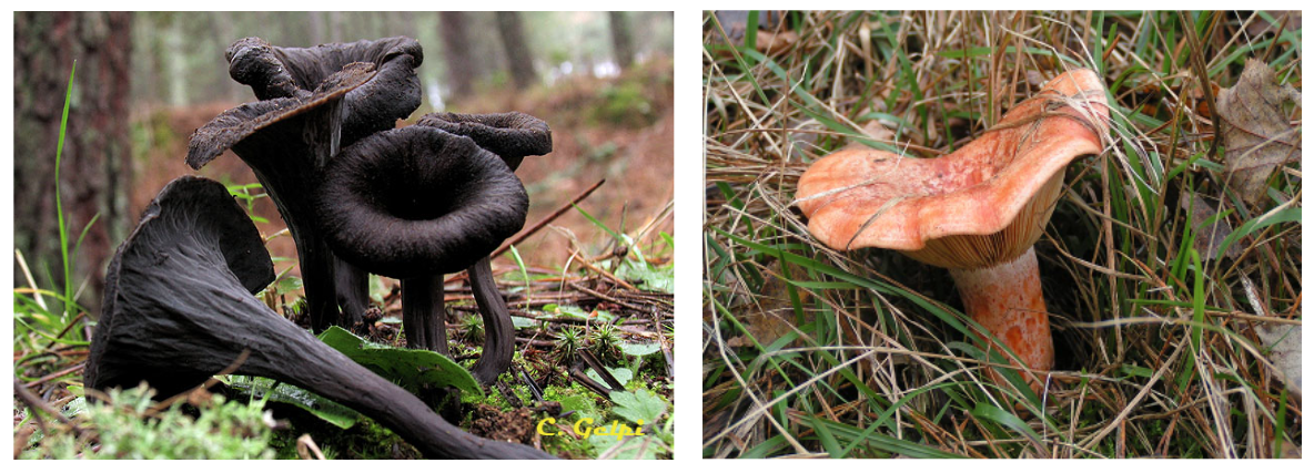
Before jumping into multiple-class image classification we will start with two different fungi species: Craterellus cornucopioides (Trompeta de la mort) and Lactarius deliciosus (Pinetell).
Gathering the data
There will be two sources of images: mushroomserver and google images. Mushroomserver is a social network from mushroom enthusiasts who upload photographs of fungis all over the world. Lucky for us a user has a public folder with photos of all the main species. Using the google_images_download python library in a small script, we can download some more images to make our dataset more robust. With both sources we gathered 504 images of Craterellus cornucopioides and 487 images of Lactarius deliciosus. Usually, thousands of images are used for this type of experiments, let’s see where we can get to with this amount.
# Import google_images_download function from library
from google_images_download import google_images_download

# Dictinoary with cientific (latin) name and common name of
# mushrooms to classify.
boletus_dictionary = {
    "Lactarius deliciosus": "Pinetell",
    "Craterellus cornucopioides": "Trompeta"
}

# Create instance of google images downloader
response = google_images_download.googleimagesdownload()

# Loop through the different fungi and donwload first
# 100 images from google.
for boletus in boletus_dictionary.keys():
    # Arguments to download
    argument = {
        "keywords": boletus,
        "limit": 100,
        "format": "jpg",
        "output_directory": "downloads/"
    }
    # Actual download
    paths = response.download(argument)
Understanding Images
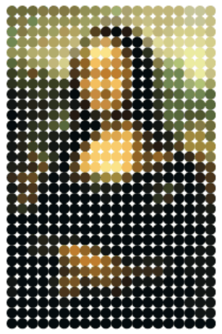
Images are made of pixels and each pixel contains colour information of specific parts of an image. The following image is a low-pixel representation of the Mona Lisa (by Leonardo Da Vinci). Although we don’t see the full set of colors represented in the original image, our brain understands the context as a whole.
To save the image information on computers it store the position of each pixel in the image and the color associated with it. For example, to represent the next grayscale image, it only stores a value between 0 and 255 (0 = completely black, 255 = completely white).
![]()
Any color can be represented as the sum of red, green and blue. Therefore, three channels (R,G and B) will be used when working with colored images. Instead of having one single matrix as the grayscale image above, we will have three different matrices: the first will be used for red, the second for green and the third in blue.
![]()
Prepare data for consumption
Images obtained have different sizes and shapes. With the following code we will resize them to be squared and with the same pixel density.
# Import walk and remove functions as helpers to manage files
from os import walk, remove
# Import skimage.io as a helper library to resize images
import skimage.io

# For each fungi in our dictionary
for boletus in boletus_dictionary.keys():
    # Get image filenames for this fungi
    filenames = next(walk("downloads/"+boletus), (None, None, []))[2]

    # For each image of this mushroom
    for i, filename in enumerate(filenames):
        try:
            # 1. read image
            image = skimage.io.imread(
                fname="downloads/"+str(boletus)+"/" +str(filename))
            # 2. resize image to 128x128x3 (3 channels rgb)
            image_resized = resize(image, (128, 128),
                           anti_aliasing=True)
            # 3. remove old image
            remove("downloads/"+str(boletus)+"/" +str(filename))
            # 4. save old image
            image = skimage.io.imsave(
                fname="downloads/"+str(boletus)+"/"+ str(i)
                    + "_" +str(boletus)+".jpg",
                arr=image_resized)
        except:
            # If something of the above did not work, remove old image anyway
            remove("downloads/"+str(boletus)+"/"+str(filename))
Next, we will define a function to split the dataset into the Training (70%), Validation (20%) and Testing (10%) set.
# Define auxiliar function to split dataset.
# Train, validate and test will contain the
# path to each image and not the image itself.
def split_dataset():

    trainSet = []
    testSet = []
    valSet = []

    # Iterate through the dictionary and save
    # 70% of images into training, 20% into
    # validation and 10% into test.
    for boletus in boletus_dictionary.keys():

        # Get all filenames for a mushroom type
        filenames = next(walk(image_path+boletus),
            (None, None, []))[2]  # [] if no file

        # Randomize selection
        np.random.shuffle(filenames)
        indicies_for_splitting = [int(len(filenames) * 0.7),
             int(len(filenames) * (0.8))]

        # Split filenames and append to sets
        subset_train, subset_test, subset_val =
            np.split(filenames, indicies_for_splitting)
        for train_name in subset_train:
            trainSet.append(image_path+boletus + "/" +train_name)
        for test_name in subset_test:
            testSet.append(image_path+boletus + "/"+test_name)
        for val_name in subset_val:
            valSet.append(image_path+boletus + "/"+val_name)

    # Print set lenght
    print("train: " + str(len(trainSet)))
    print("test: " + str(len(testSet)))
    print("val: " + str(len(valSet)))

    # Shuffle all different fungi in the set
    np.random.shuffle(trainSet)
    np.random.shuffle(testSet)
    np.random.shuffle(valSet)

    return trainSet, testSet, valSet
The number of images in the dataset is quite small (991). A common trick is to apply small transformations to the images to obtain a bigger dataset. This technique is called image augmentation. In this project we will perform the following transformations:
- Flip the image horizontally.
- Apply noise to the image (change the value of some pixels).
- Rotate the image from -45 to 45 degrees.
# Auxiliar function inside our data generator to load an image
def _load_image_(self,theIndex):

        # Get the name of the image to load
        name = self.fileNames[theIndex].split("_")[1].split(".")[0]

        # Load the image
        theImage = io.imread(self.fileNames[theIndex])

        # Transform image to floating point
        theImage = img_as_float(theImage)

        # Transform image randomly

        # Flip?
        if bool(random.getrandbits(1)):
            theImage = np.fliplr(theImage)

        # Noise?
        if bool(random.getrandbits(1)):
            theImage = random_noise(theImage)

        # Rotate?
        if bool(random.getrandbits(1)):
            degree = random.randint(-45, 45)
            theImage = rotate(theImage, degree)

        # Set class to 1 if lactarius 0 otherwise
        if "Lactarius" in name:
            theClass = 1
        else:
            theClass = 0

        return theImage,theClass
Simple Neural Network
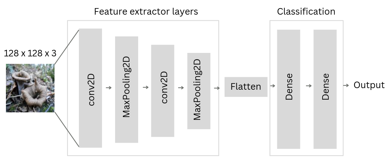
The neural network architecture used to classify images has the following parts:
- Feature extractor. This layer is in charge to transform the input image into a small representation using consecutive layers (CNN and pooling).
- Classifier. This layer uses the output from the feature extractor to classify the image. Normally, it is composed by a flattening layer (transforms the output into a 1D tensor) and some fully connected layers. The last layer will represent the output class.
The layers used for this experiments are the following:
# from keras import layers, models and optimizers
from tensorflow.keras import models
from tensorflow.keras import optimizers
from tensorflow.keras.layers import Conv2D, MaxPooling2D,Dense, Flatten

theModel=models.Sequential([
        # Feature extractor layers
        Conv2D(32,(3,3),activation='relu',input_shape=(128,128,3)),
        MaxPooling2D((2,2),padding='same'),
        Conv2D(32,(3,3),activation='relu'),
        MaxPooling2D((2,2),padding='same'),

        # Flatten before starting with classification layers
        Flatten(),

        # Classification layer with 128 neurons
        Dense(128, activation='relu'),

        # Last classification layer with 1 output neuron (only 2 classes)
        Dense(1,activation='sigmoid')
    ])
Every time a neural network finishes passing a batch through the network and generating prediction results, it must decide how to use the difference between the results it got and the values it knows to be true to adjust the weights on the nodes so that the network steps towards a solution. The algorithm that determines that step is known as the optimization algorithm. For this example we will use RMSprop (a correction to Adagrad) with a small learning rate (0.0001).
The purpose of loss functions is to compute the quantity that a model should seek to minimize during training. Binary crossentropy computes the cross-entropy loss between true labels and predicted labels.
# Set up the optimizer
opt = optimizers.RMSprop(learning_rate=0.0001)

# And compile the model
theModel.compile(loss='binary_crossentropy', optimizer=opt,
    metrics=['accuracy', 'binary_accuracy'])
With everything prepared, let’s fit the model!
# Split dataset
trainSet, testSet, valSet = split_dataset()

# Use the data generator with image augmentation for train set
trainGenerator=DataGenerator(fileNames=trainSet,encoder=encoder,
    doRandomize=True)
testGenerator=DataGenerator(fileNames=testSet,encoder=encoder,
    doRandomize=False)
valGenerator=DataGenerator(fileNames=valSet,encoder=encoder,
    doRandomize=False)

# Fit the model
trainHistory = theModel.fit(x=trainGenerator,
    validation_data=valGenerator, epochs=100, verbose=2)
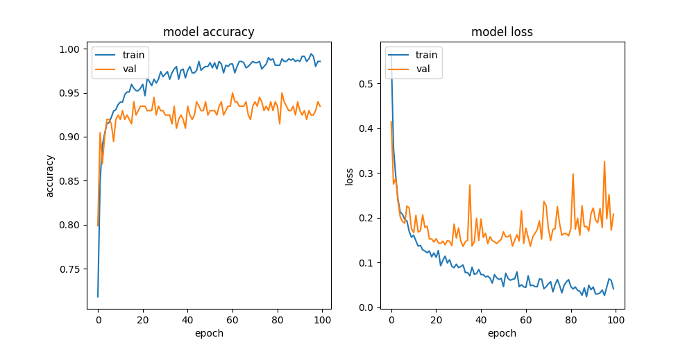
Fit function returns train history with valuable information and it can be used to detect if there is a case of overfitting. The following figure is a plot of our train history. Even using image augmentation the gap between validation and train accuracy indicates we have overfitting in our model. Let’s see how we can solve it!
Transfer learning
Transfer learning consists of taking features learned on one problem, and leveraging them on a new, similar problem. It is usually done for tasks where your dataset has too little data to train a full-scale model from scratch. The most common incarnation of transfer learning in the context of deep learning is the following workflow:
- Take layers from a previously trained model.
- Freeze them, so as to avoid destroying any of the information they contain during future training rounds.
- Add some new, trainable layers on top of the frozen layers. They will learn to turn the old features into predictions on a new dataset.
- Train the new layers on your dataset.
- Fine tunning (optional step). Consists of unfreezing the entire model you obtained above (or part of it), and re-training it on the new data with a very low learning rate. This can potentially achieve meaningful improvements, by incrementally adapting the pretrained features to the new data (possible overfitting).
For our project we will use pre-trained feature extractor layers and add classification layers on top of it. The final architecture will look like this:
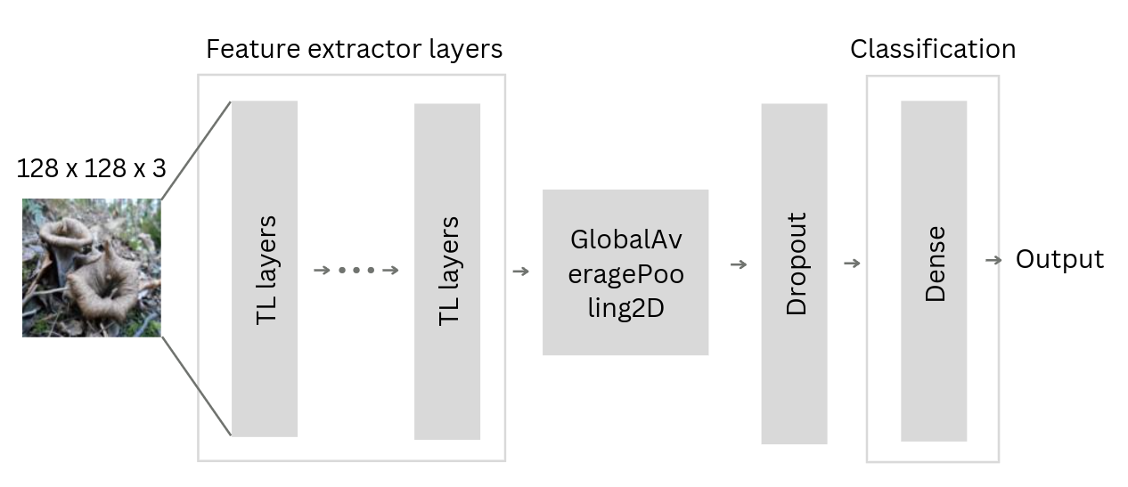
And the new architecture will be defined like this:
# import applications from keras
from tensorflow.keras import applications

# base will have an input shape = 128x128x3
# weights will come from imagenet db
# and top will not be included (we will add our own)
base = applications.Xception(
    input_tensor=layers.Input(shape=(128,128,3)),
    weights='imagenet',
    include_top=False,
)

# finally, set weights as not trainable
base.trainable = False

theModel=models.Sequential([
        # Input shape
        tf.keras.Input(shape=(128, 128, 3)),
        # Add transfer learning layers
        base,
        # Convert features of shape to vectors
        GlobalAveragePooling2D(),
        # Add 0.2 dropout to avoid overfitting
        Dropout(0.2),
        # Append a simple classification layer of 1 neuron
        Dense(1,activation='sigmoid')
    ])

# define the optimizer
opt = optimizers.Adam()

# and compile the model
theModel.compile(
    loss=tf.keras.losses.BinaryCrossentropy(from_logits=True),
    optimizer=opt,
    metrics=['accuracy', 'binary_accuracy'])
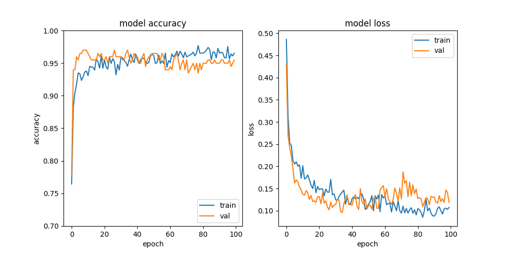
History plot of the new neural network using transfer learning shows a better convergence. We have achieved a big reduction of the previous overfitted model!
Evaluation
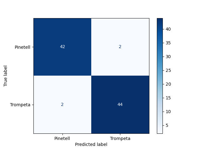
Evaluation is performed with the transfer learning model and the test Dataset. The confusion matrix obtained is shown below with a sensitivity of 0.955 and a specificity of 0.957. This means that for both Craterellus cornucopioides and Lactarius deliciosus our model identifies correctly the specie 95% of times.
Conclusion
Gathering the data, preparing it for consumption, designing a basic neural network for image classification and finally using transfer learning to avoid overfitting. The purpose of this project was to demonstrate how to build a reliable model with a small data set (~ 500 images per class). In future chapters, we will work with more than two classes, making it a multi-class classifier.