
Metrics are the key to the evaluation. In essence, a metric will give a score to our model based on the error of the predictions. Therefore, metrics can be used to compare different models and determine which will yield better results. There are several known metrics that we will cover in this post, both for regression and classification problems. If none of this metrics suit our problem, we can always develop our own metric.
Regression
A regression problem always outputs a value. Regression metrics will compare a set of our model’s output (y) with the real values (x).
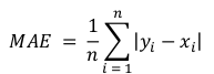
- Mean Absolute Error (MAE). As its name suggests, the MAE score is calculated as the average of the absolute error values. Absolute or abs() is a mathematical function that simply makes a number positive. Therefore, the difference between an expected and predicted value may be positive or negative and is forced to be positive when calculating the MAE. The formula is:
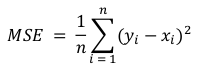
- Mean Squared Error (MSE). The MSE is calculated as the mean or average of the squared differences between predicted and expected target values in a dataset. The squaring has the effect of inflating or magnifying large errors. Therefore, when using MSE having large errors in our model will be more penalised. The formula is:
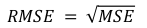
- Root Mean Squared Error (RMSE). The RMSE is an extension of the mean squared error and it is calculated by performing the square root of MSE. The units of the RMSE are the same as the original units of the target value that is being predicted, making it easy to interpret. It may be common to use MSE loss to train a regression predictive model, and to use RMSE to evaluate and report its performance. The formula is:
The following python code may be used to get the three metrics:
# Import from sklearn.metrics mean absolute error function
from sklearn.metrics import mean_absolute_error
# Import from sklearn.metrics mean absolute squared function
from sklearn.metrics import mean_squared_error

# Real value example
real_output = [1.0, 1.0, 1.0, 1.0, 1.0, 1.0, 1.0, 1.0, 1.0, 1.0, 1.0]
# Predicted value example
predicted_output = [1.0, 0.9, 0.8, 0.7, 0.6, 0.5, 0.4, 0.3, 0.2, 0.1, 0.0]

# Get MAE
mae = mean_absolute_error(real_output, predicted_output)

# Get MSE
mse = mean_squared_error(real_output, predicted_output, squared=True)

# Get RMSE
rmse = mean_squared_error(real_output, predicted_output, squared=False)
Classification
The base of any classification problem metric is the confusion matrix. A confusion matrix is a table with combinations of predicted and actual values of each class. In a very simple binary classification problem, the confusion matrix may look like this:
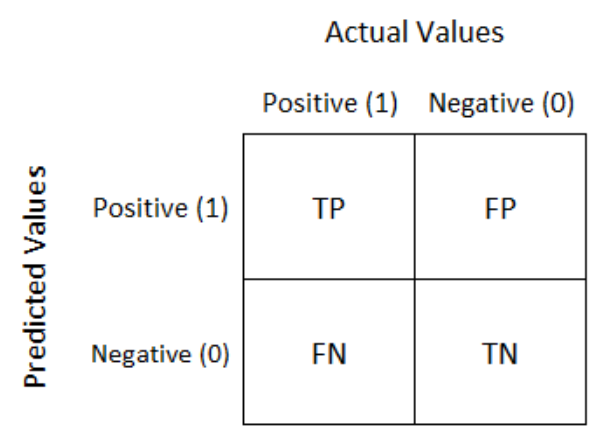
Where values of each cell indicate true positive (TP), false positive (FP), false negative (FN) and true negative (TN). Different classification metrics can be calculated using confusion matrix values:
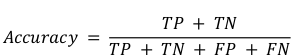
- Accuracy. Simply measures how often the classifier correctly predicts. It is useful when the target class is well balanced but is not a good choice for the unbalanced classes. Accuracy result may be misleading as it only takes into account correct predictions. The formula is:
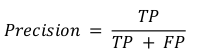
- Precision. Explains how many of the correctly predicted cases actually turned out to be positive. Precision is useful in the cases where False Positive is a higher concern than False Negatives. The formula is:
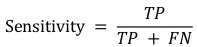
- Sensitivity. Explains how many of the actual positive cases we were able to predict correctly with our model. It is a useful metric in cases where False Negative is of higher concern than False Positive. The formula is:
- Specificity. Explains the probability of a negative test, conditioned on truly being negative. It is a useful metric in cases where True Negative is of higher concern than True Positive. The formula is:
